Rstykt

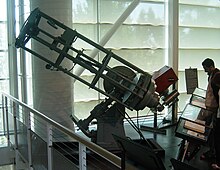
George Ritchey's 24-inch (0.6 m) reflecting telescope, the first RCT to be built, later on display at the Chabot Space and Science Center in 2004

A Ritchey–Chrétien telescope (RCT or simply RC) is a specialized variant of the Cassegrain telescope that has a hyperbolic primary mirror and a hyperbolic secondary mirror designed to eliminate off-axis optical errors (coma). The RCT has a wider field of view free of optical errors compared to a more traditional reflecting telescope configuration. Since the mid 20th century, a majority of large professional research telescopes have been Ritchey–Chrétien configurations; some well-known examples are the Hubble Space Telescope, the Keck telescopes and the ESO Very Large Telescope.

History

The 40-inch (1.0 m) Ritchey at United States Naval Observatory Flagstaff Station

The Ritchey–Chrétien telescope was invented in the early 1910s by American astronomer George Willis Ritchey and French astronomer Henri Chrétien. Ritchey constructed the first successful RCT, which had a diameter aperture of 60 cm (24 in) in 1927 (e.g. Ritchey 24-inch reflector). The second RCT was a 102 cm (40 in) instrument constructed by Ritchey for the United States Naval Observatory; that telescope is still in operation at the Naval Observatory Flagstaff Station.

Design

The basic Ritchey–Chrétien two-surface design is free of third-order coma and spherical aberration,^[1] although it does suffer from fifth-order coma, severe large-angle astigmatism, and comparatively severe field curvature.^[2] The remaining aberrations of the basic design may be improved with the addition of smaller optical elements near the focal plane.^[3][4] When focused midway between the sagittal and tangential focusing planes, stars are imaged as circles, making the RCT well suited for wide field and photographic observations. As with the other Cassegrain-configuration reflectors, the RCT has a very short optical tube assembly and compact design for a given focal length. The RCT offers good off-axis optical performance, but the Ritchey–Chrétien configuration is most commonly found on high-performance professional telescopes.

A telescope with only one curved mirror, such as a Newtonian telescope, will always have aberrations. If the mirror is spherical, it will suffer from spherical aberration. If the mirror is made parabolic, to correct the spherical aberration, then it must necessarily suffer from coma and astigmatism. With two non-spherical mirrors, such as the Ritchey–Chrétien telescope, coma can be eliminated as well. This allows a larger useful field of view. However, such designs still suffer from astigmatism. This too can be cancelled by including a third curved optical element. When this element is a mirror, the result is a three-mirror anastigmat. Alternatively, a Ritchey-Chrétien may use one or several low-power lenses in front of the focal plane as a field-corrector to correct astigmatism and flatten the focal surface, as for example the SDSS telescope and the VISTA telescope; this can allow a field-of-view up to around 3 degrees diameter.

(Although the Schmidt camera can deliver even wider fields up to about 7 degrees, the Schmidt requires a full-aperture corrector plate which restricts it to apertures below 1.2 metres, while a Ritchey-Chrétien can be much larger).

In practice, each of these designs may also include any number of flat fold mirrors, used to bend the optical path into more convenient configurations.

In a Ritchey-Chrétien design, as in most Cassegrain systems, the secondary mirror blocks a central portion of the aperture. This ring-shaped entrance aperture significantly reduces a portion of the modulation transfer function (MTF) over a range of low spatial frequencies, compared to a full-aperture design such as a refractor.^[5] This MTF notch has the effect of lowering image contrast when imaging broad features. In addition the support for the secondary (the spider) may introduce diffraction spikes in images.

Mirror parameters

Diagram of a Ritchey-Chrétien reflector telescope

The radii of curvature of the primary and secondary mirrors, respectively, in a two-mirror Cassegrain configuration are

R1=−2DFF−B{displaystyle R_{1}=-{frac {2DF}{F-B}}}

and

R2=−2DBF−B−D{displaystyle R_{2}=-{frac {2DB}{F-B-D}}}

where

• 
  F{displaystyle F} is the effective focal length of the system,


• 
  B{displaystyle B} is the back focal length (the distance from the secondary to the focus), and


• 
  D{displaystyle D} is the distance between the two mirrors.

If, instead of B{displaystyle B} and D{displaystyle D}, the known quantities are the focal length of the primary mirror, f1{displaystyle f_{1}}, and the distance to the focus behind the primary mirror, b{displaystyle b}, then D=f1(F−b)/(F+f1){displaystyle D=f_{1}(F-b)/(F+f_{1})} and B=D+b{displaystyle B=D+b}.

For a Ritchey–Chrétien system, the conic constants K1{displaystyle K_{1}} and K2{displaystyle K_{2}} of the two mirrors are chosen so as to eliminate third-order spherical aberration and coma; the solution is

K1=−1−2M3⋅BD{displaystyle K_{1}=-1-{frac {2}{M^{3}}}cdot {frac {B}{D}}}

and

K2=−1−2(M−1)3[M(2M−1)+BD]{displaystyle K_{2}=-1-{frac {2}{(M-1)^{3}}}left[M(2M-1)+{frac {B}{D}}right]}

where M=F/f1=(F−B)/D{displaystyle M=F/f_{1}=(F-B)/D} is the secondary magnification.^[6] Note that K1{displaystyle K_{1}} and K2{displaystyle K_{2}} are less than −1{displaystyle -1} (since M>1{displaystyle M>1}), so both mirrors are hyperbolic. (The primary mirror is typically quite close to being parabolic, however.)

The hyperbolic curvatures are difficult to test, especially with equipment typically available to amateur telescope makers or laboratory-scale fabricators; thus, older telescope layouts predominate in these applications. However, professional optics fabricators and large research groups test their mirrors with interferometers. A Ritchey–Chrétien then requires minimal additional equipment, typically a small optical device called a null corrector that makes the hyperbolic primary look spherical for the interferometric test. On the Hubble Space Telescope, this device was built incorrectly (a reflection from an un-intended surface leading to an incorrect measurement of lens position) leading to the error in the Hubble primary mirror.^[7] Incorrect null correctors have led to other mirror fabrication errors as well, such as in the New Technology Telescope.

Examples of large Ritchey–Chrétien telescopes

Ritchey intended the 100-inch Mount Wilson Hooker telescope (1917) and the 200-inch (5 m) Hale Telescope to be RCTs. His designs would have provided sharper images over a larger usable field of view compared to the parabolic designs actually used. However, Ritchey and Hale had a falling-out. With the 100-inch project already late and over budget, Hale refused to adopt the new design, with its hard-to-test curvatures, and Ritchey left the project. Both projects were then built with traditional optics. Since then, advances in optical measurement^[8] and fabrication^[9] have allowed the RCT design to take over - the Hale telescope, dedicated in 1948, turned out to be the last world-leading telescope to have a parabolic primary mirror.^[10]

16 in (41 cm) RC Optical Systems truss telescope, part of the PROMPT Telescopes array

• The 10.4 m Gran Telescopio Canarias at Roque de los Muchachos Observatory
  


• The two 10.0 m telescopes of the Keck Observatory
  


• The four 8.2 m telescopes comprising the Very Large Telescope in Chile
  


• The 8.2 m Subaru telescope at Mauna Kea Observatory
  


• The two 8.0 m telescopes comprising the Gemini Observatory
  


• The 4.1 m Visible and Infrared Survey Telescope for Astronomy at the Paranal Observatory (Chile)


• The 4.0 meter Mayall Telescope at Kitt Peak.


• The 4.0 meter Blanco telescope at the Cerro Tololo Inter-American Observatory, Chile.


• The 3.9 m Anglo-Australian Telescope at Siding Spring Observatory (Australia)


• The 3.6 m Devasthal Optical Telescope of Aryabhatta Research Institute of Observational Sciences, Nainital, India.


• The 3.58 m New Technology Telescope at the European Southern Observatory
  


• The 3.58 m Telescopio Nazionale Galileo at Roque de los Muchachos Observatory
  


• The 3.5 m ARC telescope at Apache Point Observatory, New Mexico, U.S.


• The 3.5 m Calar Alto Observatory telescope at mount Calar Alto (Spain)


• The 3.5 m Herschel Space Observatory currently operating in orbit at the L2 point 1.5 million km from Earth


• The 3.50 m WIYN Observatory at Kitt Peak National Observatory
  


• The 3.4 m INO340 Telescope at Iranian National Observatory (Iran)


• The 2.65 m VLT Survey Telescope at ESO’s Paranal Observatory
  


• The 2.56 m effective f/11 Nordic Optical Telescope on La Palma, Canary Islands.


• The 2.50 m Sloan Digital Sky Survey telescope (modified design) at Apache Point Observatory, New Mexico, U.S.


• The 2.4 m Hubble Space Telescope currently in orbit around the Earth


• The 2.4 m Thai National Observatory telescope on Doi Inthanon, Thailand


• The 2.2 m Calar Alto Observatory telescope at mount Calar Alto (Spain)


• The 2.15 m Leoncito Astronomical Complex telescope on San Juan, Argentina.


• The 2.1 m telescope at San Pedro Martir, National Astronomical Observatory (Mexico)
  


• The 2.0 m Liverpool Telescope (robotic telescope) on La Palma, Canary Islands
  


• The 2.0 m telescope at Rozhen Observatory
  


• The 2.0 m Himalayan Chandra Telescope of the Indian Astronomical Observatory, Hanle, India


• The 1.8 m Pan-STARRS telescopes at Haleakala on Maui, Hawaii
  


• The 1.65 m telescope at Molėtai Astronomical Observatory, Lithuania
  


• The 1.6 m Mont-Mégantic Observatory telescope on Mont-Mégantic in Quebec, Canada
  


• The 1.0 m Ritchey Telescope at the United States Naval Observatory Flagstaff Station (the final telescope made by G. Ritchey before his death)


• The 1.0 m DFM Engineering f/8 at Embry-Riddle Observatory in Daytona Beach, Florida
  


• The 0.85 m Spitzer Space Telescope, infrared space telescope currently operating in Earth-trailing orbit


• The 0.208 m LOng Range Reconnaissance Imager (LORRI) camera on board the New Horizons space craft, currently beyond Pluto

See also

Wikimedia Commons has media related to Ritchey-Chrétien telescopes.

• List of largest optical reflecting telescopes


• List of telescope types


• Reflecting telescope


• Schmidt–Cassegrain telescope


• Maksutov telescope

References

^
Sacek, Vladimir (14 July 2006). "Classical and aplanatic two-mirror systems". Notes on Amateur Telescope Optics. Retrieved 2010-04-24..mw-parser-output cite.citation{font-style:inherit}.mw-parser-output q{quotes:"""""""'""'"}.mw-parser-output code.cs1-code{color:inherit;background:inherit;border:inherit;padding:inherit}.mw-parser-output .cs1-lock-free a{background:url("//upload.wikimedia.org/wikipedia/commons/thumb/6/65/Lock-green.svg/9px-Lock-green.svg.png")no-repeat;background-position:right .1em center}.mw-parser-output .cs1-lock-limited a,.mw-parser-output .cs1-lock-registration a{background:url("//upload.wikimedia.org/wikipedia/commons/thumb/d/d6/Lock-gray-alt-2.svg/9px-Lock-gray-alt-2.svg.png")no-repeat;background-position:right .1em center}.mw-parser-output .cs1-lock-subscription a{background:url("//upload.wikimedia.org/wikipedia/commons/thumb/a/aa/Lock-red-alt-2.svg/9px-Lock-red-alt-2.svg.png")no-repeat;background-position:right .1em center}.mw-parser-output .cs1-subscription,.mw-parser-output .cs1-registration{color:#555}.mw-parser-output .cs1-subscription span,.mw-parser-output .cs1-registration span{border-bottom:1px dotted;cursor:help}.mw-parser-output .cs1-hidden-error{display:none;font-size:100%}.mw-parser-output .cs1-visible-error{font-size:100%}.mw-parser-output .cs1-subscription,.mw-parser-output .cs1-registration,.mw-parser-output .cs1-format{font-size:95%}.mw-parser-output .cs1-kern-left,.mw-parser-output .cs1-kern-wl-left{padding-left:0.2em}.mw-parser-output .cs1-kern-right,.mw-parser-output .cs1-kern-wl-right{padding-right:0.2em}
Rutten, Harrie; van Venrooij, Martin (2002). Telescope Optics. Willmann-Bell. p. 67. ISBN 0-943396-18-2.
^ Bowen, I. S., and A. H. Vaughan (1973). "The optical design of the 40-in. telescope and of the Irenee DuPont telescope at Las Campanas Observatory, Chile". Applied Optics. 12 (77): 1430–1435. Bibcode:1973ApOpt..12.1430B. doi:10.1364/AO.12.001430.CS1 maint: Multiple names: authors list (link)
Harmer, C. F. W.; Wynne, C. G. (October 1976). "A simple wide-field Cassegrain telescope". Monthly Notices of the Royal Astronomical Society. 177: 25–30. Bibcode:1976MNRAS.177P..25H. doi:10.1093/mnras/177.1.25P. Retrieved 29 August 2017.
^ "THE EFFECTS OF APERTURE OBSTRUCTION".
Smith, Warren J. (2008). Modern Optical Engineering (4th ed.). McGraw-Hill Professional. pp. 508–510. ISBN 978-0-07-147687-4.
Allen, Lew; et al. (1990). The Hubble Space Telescope Optical Systems Failure Report (PDF). NASA. NASA-TM-103443.
^ Burge, J.H. (1993). "Advanced Techniques for Measuring Primary Mirrors for Astronomical Telescopes" (PDF). Ph.D. Thesis, University of Arizona.
^ Wilson, R.N. (1996). Reflecting Telescope Optics I. Basic Design Theory and its Historical Development. 1. Springer-Verlag: Berlin, Heidelberg, New York. P. 454
^ Zirker, J.B. (2005). An acre of glass: a history and forecast of the telescope. Johns Hopkins Univ Press., p. 317.